Introduction to Artificial Neural Networks

Introduction

This guide will serve as an introduction to ANNs. We will build a neural network from scratch without using any specialised libraries like keras or pytorch. We will only use NumPy for matrix operations and other maths functions.

The best way to learn about ANN is to solve a real world problem. We will try to solve a classification problem using a neural network.

The Problem

We will be tackling the problem of digit classification. We will be given a grayscale image of a handwritten digit (between 0 and 9) and our goal is to correctly identify it. This is a beginner level problem and is ideal for understanding the workings of a neural net.

The dataset that we will use is known as MNIST dataset. It is provided on Kaggle. Use the link below to download it. MNIST dataset

About the Dataset

The dataset consists of thousands of images of handwritten digits. Each image is grayscale, and it has fixed dimensions of 28x28 pixels. So all in all, each image is 784 pixels of values ranging from 0 to 255. Since all the images are grayscale, we need not worry about pixel colours. Each pixel can only have values between 0 and 255.

Matrix Representations

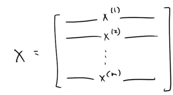
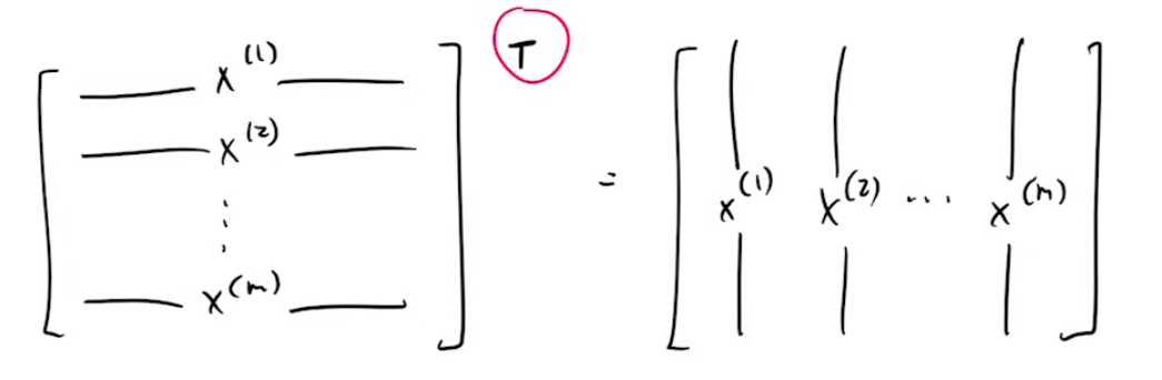
Lets assume we have m images. If we represent our dataset as a matrix, then we have a matrix of dimensions m x 784, where rows are representing the number of images and columns are representing the number of pixels in each image. Let’s denote this matrix by X.

We will now take transpose of this matrix. We do this so that future calculations are made easy for us. This is a completely optional step and it’s only purpose is ease of calculations. So, now we have a matrix of dimensions 784 x m, where each image is now represented in a column instead of a row.

Architecture

We will build a very simple neural network that will only have 3 layers in total. The 0th layer is called the input layer, and the last layer is called the output layer. Since, input layer neurons do not have any calculations associated with them, we say that our model only has 2 computational layers, i.e., 1 hidden and 1 output.

The input layer will consist of 784 neurons, representing 784 pixels in an image. The hidden layer will have 10 neurons, and the output layer will also have 10 neurons, representing the digits 0 to 9. And so, our model diagram will look something like this :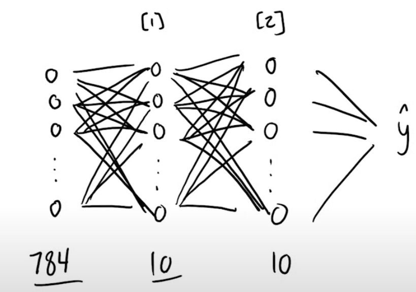

We have chosen to use 10 neurons simply because it works well enough in our case. We could have gone for more neurons in the hidden layer, and could have added more hidden layers as well, but it is unnecessary for our dataset.

Notations

Every layer will have inputs and outputs, but the input of a layer will always be the final output of a previous layer. So we define 2 outputs, immidiate output, and final output. They are denoted in the following way:

• Immidiate output of a layer is denoted using Z^[n]. This means the current output of nth layer.
  For the first layer of our ANN, it is just the input matrix of dimensions (784 x m).
  For second layer of our ANN, it will be a matrix of dimensions (10 x m), as this layer only has 10 neurons.
  For the third and final layer of our ANN, this will again be a matrix of dimensions (10 x m) as we have 10 possible classes.
  General formula for denoting output is:

Z^[n]

• Final output of a layer is denoted by A^[n]. This means the final output, after applying activation function, of nth layer.
  For the first layer of our ANN, it will be the same as the input matrix of dimensions (784 x m).
  For second layer of our ANN, it will be a matrix of dimensions (10 x m), as this layer only has 10 neurons.
  For the third and final layer of our ANN, this will again be a matrix of dimensions (10 x m) as we have 10 possible classes.
  General formula for denoting output is:

A^[n] = σ(W^[n] . Z^[n] + b^[n])

Where, W^[n] represents weight matrix of the nth layer, b^[n] represents the bias matrix of the nth layer, σ represents the activation function.

Training an ANN

There are 3 parts to training a neural net.

1. Activation functions : Introduce non linearity and provide threshold for neurons in the neural net.
2. Forward propagation : Take an input image > run through the network > compute the output.
3. Back propagation : Feedbacks from the difference between network’s output and label.

Activation function

We introduce a non-linearity in our hidden layer. Otherwise our neural net will only calculate a linear combination of values and behaves like linear regression regardless of the number of hidden layers.

In simpler terms, activation functions provide a threshold value, only above which will the neuron be fired. This means that if the calculated value of a neuron does not match the threshold, then instead of passing the value, it will pass on a zero.

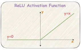
There are a number of activation functions available, like, sigmoid, tan h, ReLU, etc. In our model, we will use ReLU(x). It stands for Rectified Linear Unit and is defined as:

ReLU(x) = x, x > 0
          0, x ≤ 0

Every layer after the input layer is going to have activation function applied to it. This can be denoted as:

A^[x] = σ(Z^[x])

In our ANN, σ = ReLU,     for the hidden layer
                softmax,  for the output layer

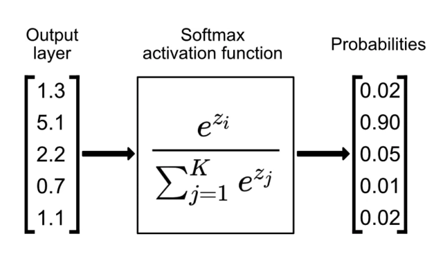
softmax function serves 2 benefits:

• it converts the raw output of a neural net into a vector of probabilities with values lying between 0 and 1. This essentially provides us with a probability distribution over the expected output classes. In our case, we have 10 possible output classes (digits 0 to 9). So, for a 784 pixel input image, we get a probability of that image being one of the 10 digits.
• it amplifies the difference between probabilities. e^{(small value)} tends to 0, while e^{(large value)} tends to infinite.

Forward propagation

After deciding the activation function, we are now ready to start training the neural net. These 2 steps, (forward and back propagation) are done in a loop, to train the model. For understanding purposes, we will considering passing a single image through the network.

• Layer 1 of our ANN (input layer)
  

  • The input is going to be (784 x 1) matrix representing 1 image:
    Z^[0] = X

  • The output will also be same, since no computation is applied on this layer:
    A^[0] = X

• Layer 2 of our ANN (hidden layer)
  

  • The input will be the output of the previous layer, a (784 x 1) matrix:
    Z^[1] = A^[0] = X

  • The output will be computed and ReLU activation function will be applied. This produces a (10 x 1) matrix:
    A^[1] = ReLU (W^[1] . Z^[1] + b^[1])

• Layer 3 of our ANN (output layer)
  

  • The input will be the output of the previous layer, a (10 x 1) matrix:
    Z^[2] = A^[1]

  • The output will be computed and softmax activation function will be applied. This produces a (10 x 1) matrix:
    A^[2] = softmax (W^[2] . Z^[2] + b^[2])

Initially, the matrices, W^[1], W^[2], B^[1], B^[2] will have random values. They will be adjusted automatically by our back propagation algorithm.

Back propagation

This is used to adjust the weights and biases of the layers based on the feedback received from the output.
We get the prediction from our neural net and then by matching it to our labeled dataset, we get the deviation/error. Then, the model adjusts the weights and biases based on their contribution to the deviation.

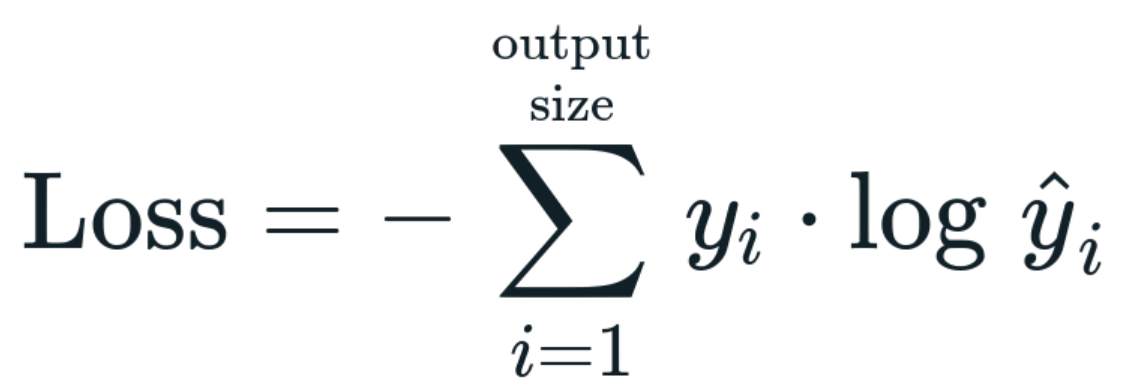
Before moving forward, we need to define our loss function. Loss functions are used to quantify the difference between predicted values of the network and actual target values.

In our case, we will use Cross-Entropy Loss Function. This is commonly used for probability distributions. It is defined as below:

We also need to define One-hot encoding : it is a method for converting categorical variables into a binary format. Let’s say, we get the image of 5 as our input. Our inputs would be 784 pixels and the label will be 5. However, we are not going to directly subtract 5 from our network’s output. Instead we perform one-hot encoding and Y for this example becomes a vector with all other labels set to 0, and 5 set to 1,

Y = [0, 0, 0, 0, 0, 1, 0, 0, 0, 0] # encoded label
                    ↑
                    5  # actual label

Now that we have our encoded labels, we can get to finding out how much our weights(W) and biases(b) contributed to the output.

To calculate the contribution of a matrix in the final output, we take the derivative of the loss function with respect to that matrix. In simpler terms, we calculate the rate of change of loss, with respect to a matrix.

Third(output) layer weights contribution

• calculate the gradient of Loss function with respect to W^[2]

dL/dW[2]	=	(∂L/∂A[2]) × (∂A[2]/∂Z[2]) × (∂Z[2]/∂W[2])
	=	(y - Y) x (A[1])T

We can see that the last term is reduced to transpose of final output of second layer. And, the first 2 terms are reduced to the difference between one-hot encoded labels(Y) and output probability distribution(y = A^[2]).

Since, we pass a total of m images, we devide the expression by m. So, the final expression becomes:

d W^[2] = (1 / m) x d (Z^[2] . A^[1]T) = (1 / m) x ( A^[2] - Y ) x (A^[1])^T

Similarly, we can get the contributions of weights and biases for all the layers.

Third(output) layer bias contribution :

d B^[2] = (1 / m) x Σ (d Z^[2]) = (1 / m) x Σ( A^[2] - Y )

Second(hidden) layer weights contribution :

d W^[1] = (1 / m) x d (Z^[1] . A^[0]T) = (1 / m) x ( W^[1]T . d Z^[2] ) . ReLU^|(Z^[1]) . A^[0]T

Note : We account for the ReLU activation function in this layer.

Second(hidden) layer bias contribution :

d B^[1] = (1 / m) x Σ (d Z^[1]) = (1 / m) x Σ( A^[1] - Y )